Overnight returns refer to the change in an asset’s price between the market’s closing level and its opening level the following morning. Even though stock exchanges are closed during these hours, the global financial system never truly sleeps.
Equity markets continue to move after the closing bell because of activity in futures markets, which trade almost 24 hours a day. These futures contracts track major indexes like the S&P 500 and Nasdaq 100 and respond instantly to news around the world as well as movements in global financial markets in Asia and Europe. When the North American markets open the next day, these changes are reflected in stock prices.
Why Overnight Returns matter
Overnight returns are an important source of long-term stock price appreciation that is often overlooked. In fact, studies including research from the Federal Reserve Bank of New York[1] show that over time, the majority of stock market gains occurred overnight, not during the trading day. These moves are often driven by factors such as:
Company-specific news: Material information (read: “market moving”) such as earnings results, merger activity, and regulatory action is typically released after the close or before the open
Economic data: Reports like inflation and jobs numbers are often published before U.S. markets open
Global events: Political, policy, or economic news can move markets outside of trading hours
Importantly, these moves can be significant, and investors who are not invested or exposed overnight can miss out on a meaningful part of total returns.
Don’t Sleep on Overnight Returns
Overnight returns can be triggered by a single news announcement, creating sharp changes as trading begins. For example, on Sunday, May 11, 2025, the White House announced major progress on trade negotiations with China, including a 90-day truce. By the time U.S. markets opened the next morning, the S&P 500 had already jumped over +3%[2]vs. the previous night’s close. That entire move happened before investors could trade stocks during normal hours, and anyone not exposed/invested overnight missed it.
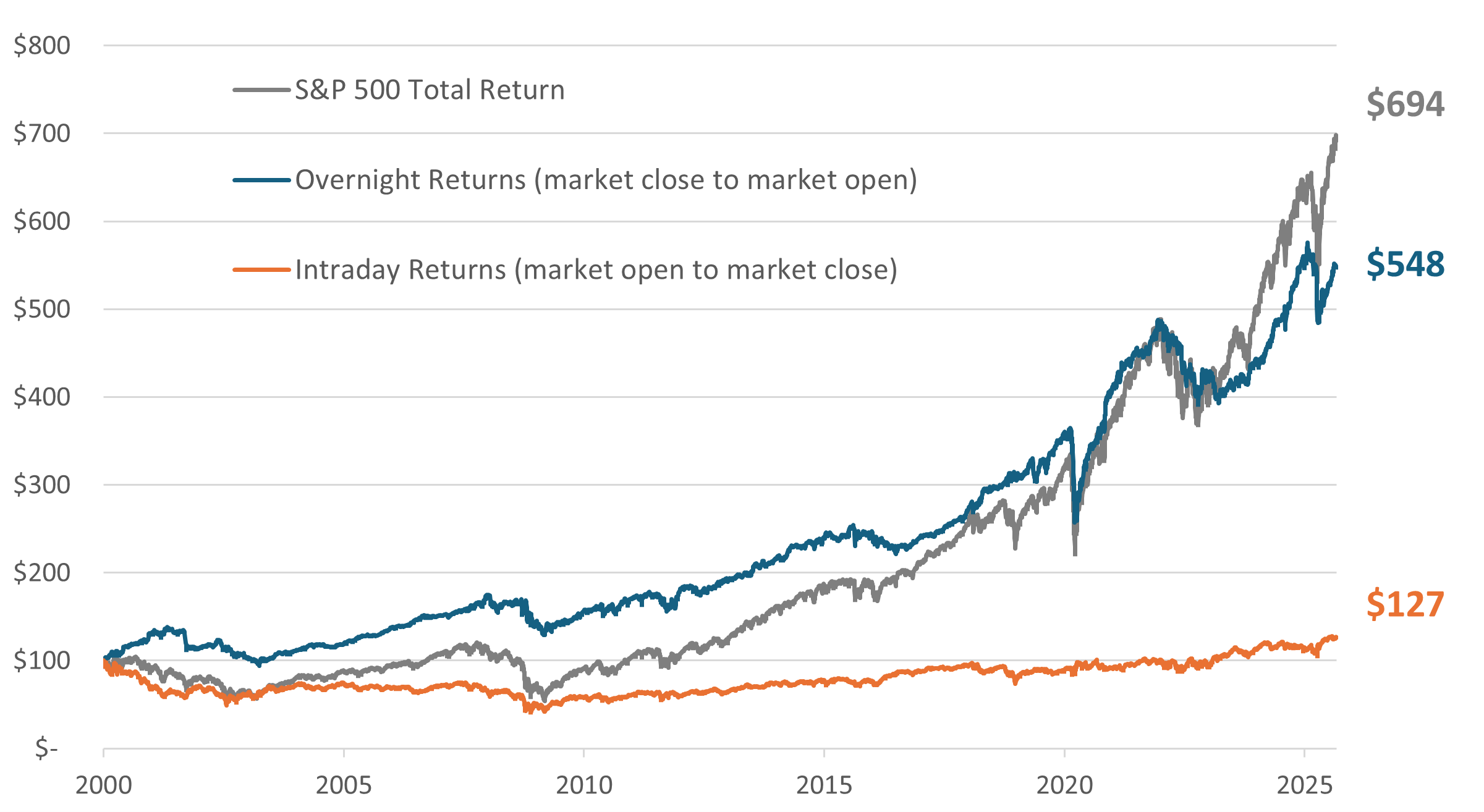
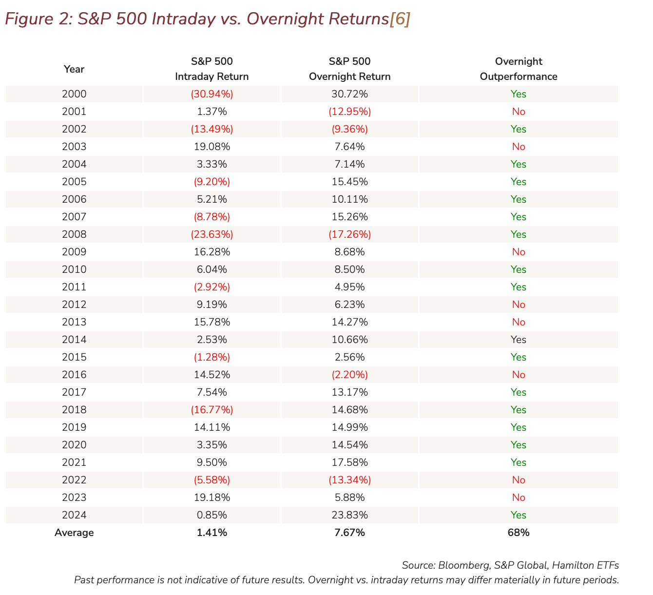
Looking at the bigger picture, overnight returns accounted for the majority of long-term market performance. Since 2000, the S&P 500 has delivered far stronger returns overnight than during the trading day. On average, annualized overnight returns were +7.67%, compared to just +1.41% during standard trading hours[3]. Put another way, a $100 investment in the S&P 500 held only during the day would have grown to about $127, while the same investment held only overnight would have grown to about $548 (Figure 1, 2).
As noted, overnight returns have historically accounted for the majority of positive market gains in the S&P 500. For vanilla equity investors, if they stayed invested overnight, they maintain that exposure. For a covered call ETF investor, the upside capture overnight can be limited by the call option. By selling call options each morning that expire at the same-day market’s close, DayMAX™ ETFs only limit upside during regular trading hours, when the upside has historically been more limited, and they are fully exposed overnight, when there has historically been more money to be made (see charts below).
Figure 1: S&P 500 Intraday vs. Overnight Returns[5]
Source: Bloomberg, S&P Global, Hamilton ETFs
Past performance is not indicative of future results. Overnight vs. intraday returns may differ materially in future periods.
Source: Bloomberg, S&P Global, Hamilton ETFs Past performance is not indicative of future results. Overnight vs. intraday returns may differ materially in future periods.
DayMAX™ ETFs: Daily Options + Overnight Returns
DayMAX™ ETFs are built to generate frequent income while maintaining exposure to overnight returns. Unlike traditional covered call strategies that write options for weeks or months, DayMAX™ ETFs sell daily (specifically, zero-days-to expiration, or 0DTE) index call options each morning that expire at the market’s close. This structure means: Continue Reading…
The Federal Reserve (the “Fed”) was founded on December 23, 1913, as the central banking system of the United States.
At the time, the U.S. had contended with a series of financial crises that had rattled the domestic economy. This included the panic of 1907: a financial crisis that was triggered by the failed attempt in October 1907 to corner the market on the stock of the United Copper Company. These panics led to bank runs, reaffirming the desire of policy makers to have central control of the monetary system.
In this piece, we review the role of the Fed and how this U.S. central bank chooses its chairperson, presidents, and determines voting power. After that, we review how these factors could impact rate decisions through 2025 and beyond, and what Harvest ETFs may be impacted by these developments and policy shifts.
The role of the Fed
Upon its founding, the U.S. Congress established three key goals for monetary policy in the Federal Reserve Act. The Fed’s statutory mandate is as follows:
Maximum Employment
Stable Prices
Moderate Long-Term Interest Rates
The Fed has many tools at its disposal to achieve these goals. More traditional monetary policy involves the utilization of open market operations, reserve requirements, and discount window lending.
Traditional monetary policy
Open market operations (OMOs)
Open market operations involve influencing the supply of balances in the federal funds market. In other words, this empowers the central bank to control the supply of money and credit in the economy.
Before the 2007-2008 housing crisis, and the global financial crisis that followed, OMOs were used to adjust the supply of reserve balances. This was done to keep the federal funds rate, which is the interest rate at which depository institutions lend reserve balances to other depository institutions overnight, at or around the target established by the Federal Open Market Committee (FOMC).
This approach evolved significantly in the wake of the 2007-2008 financial crisis and the Great Recession. In 2008, the FOMC established a near-zero target range for the federal funds rate. That move, paired with large-scale asset purchases – which we will cover later – made the Fed a target of scrutiny to a degree not seen since its founding in the early 20th century.
Reserve requirements
The Federal Reserve Act authorizes the Fed board to establish reserve requirements within a specific range. That allows the Fed to effectively implement monetary policy on certain types of deposits and other liabilities of depository institutions. In order to reach the dollar amount of a depository institutions reserve requirement, the Fed applies the reserve requirement ratios to an institutions’ reservable liabilities. After that, the Fed board is authorized to impose reserve requirements on transaction accounts, nonpersonal time of deposits, and Eurocurrency liabilities.
Discount window lending
Another important role of the Fed is discount window lending. The Fed is authorized to lend to depository institutions. Through this, the central bank can support the liquidity and stability of the domestic banking system as well as the effective implementation of monetary policy. The discount window aids depository institutions in the managing of their liquidity risks. This, in turn, helps to avoid actions that could have negative consequences for their customers. Essentially, the discount window supports the flow of credit to households and businesses.
Nontraditional monetary policy
Forward guidance
Central banks around the world use forward guidance to tell the public about the future course of monetary policy. When the Fed provides forward guidance, it allows individuals and businesses to make decisions based on that information. Because of its impact on spending and investment decision making, forward guidance influences financial and economic conditions.
The FOMC began providing forward guidance statements following its meetings in the early 2000s.
Large-scale asset purchases
Historically, outright purchases or sales of Treasury securities were used as a tool to manage the supply of bank reserves. This was done to maintain conditions in line with the federal funds target rate.
However, the global financial crisis in 2007-2008 led to dramatic changes in how the Fed approaches large-scale asset purchases. From 2008 to 2014, the FOMC authorized three rounds of large-scale asset purchase programs – also referred to as quantitative easing – as well as a maturity extension program.
The COVID-19 pandemic also presented a significant challenge for policymakers. In March 2020, the Fed launched large-scale asset purchases of U.S. Treasury securities to address the market disruptions at the beginning of the pandemic. Other steps including the launch of market functioning purchases of Treasuries and other securities. These purchases were without precedent. Asset purchases reached nearly $2 trillion of notes and bonds purchased just in 2020.
Fed presidents and voting power
The Fed is run by seven governors that are nominated by the President and confirmed by the Senate. All seven of the governors vote at every FOMC meeting. A full term for Fed governors is 14 years, and one term begins every two years. This occurs on February 1 of even-numbered years. After serving a full term, a member cannot be reappointed, whereas a member who completes an unexpired portion of a term may be reappointed.
However, if a member retires earlier, the President may appoint another governor in the interim. For example, Adriana Kugler recently resigned in August of 2025, as her term was expiring in February 2026. This seat was recently filled by the appointment and senate confirmation of Stephen Miran on September 15, 2025. It is expected he will be re-appointed this February when that term is up for renewal.
There are 12 regional bank presidents. Five of these presidents vote at a time on rotation. All 12 presidents have terms that expire at the same time with the next term expiring this coming February. The process for selecting the regional Presidents is complicated. It includes rolling terms for B and C directors of the regional bank that are intended to represent the public. The class B directors are chosen by the regional banks, and the class C directors are appointed by the Federal Reserve Board of Governors. Then, the regional banks’ Presidential nominee must be approved by the Fed’s board of seven in Washington. Chair Jerome Powell’s term as Chair is up in May of 2026 however, he has until 2028 as a board governor, although not unprecedented to serve their full terms on the board, Chairs have historically resigned from the board following their role as Chair.
While this is complicated, this has shone a spotlight on the Fed and regional banks, especially in the wake of the recent governors’ coming retirement and more so given the controversy surrounding Governor Lisa Cook and her potential dismissal.
With now three of the seven board of governors having been appointed by the current administration, should another board of governor retire, or in the case of Governor Cook be removed for cause, that move could shift voting power of the Fed , raising concerns about political influence in the realm of monetary policy. Even though there are some safeguards that remain, the perception of the Fed’s independence being weakened has the potential to unsettle markets.
Rate expectations in 2025
On Wednesday, September 17, the Fed announced that it voted to lower the target range for the federal funds rate by 0.25%, bringing the benchmark rate to 4.25%. Its decision was motivated by the moderation of economic activity in the first half of 2025, as well as slowing jobs data and the increased unemployment rate. The FOMC reiterated that it was “strongly committed to supporting maximum employment and returning inflation to its 2 percent objective.”
A September 5 report showed that the U.S. economy generated only 22,000 jobs in August. This stoked fears that the administration’s economic policies, including massive import taxes, have contributed to uncertainty in the business world. Meanwhile, the unemployment rate rose to 4.3%, moving higher than the six-month moving average. This indicates a sustained increase in unemployment.
Which Harvest ETFs are being impacted by Fed movements?
The uncertainty around Fed policy has boosted gold, benefitting two ETFs in the Harvest stable.
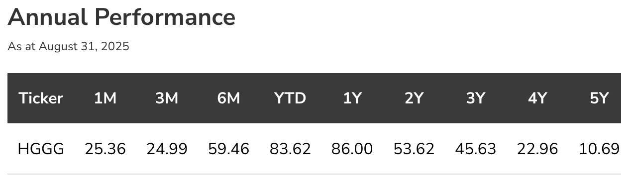
One of them is the Harvest Global Gold Giants Index ETF (TSX: HGGG), an equally weighted portfolio of the world’s leading and largest gold companies. HGGG tracks the Solactive Global Gold Giants Index TR.
Meanwhile, the shorter-term gyrations of bond prices have been a challenging environment with longer term bond prices fluctuating month over month. Mid-duration bonds have been steadier, despite upward moves in yields in August, they will continue to be data dependent.
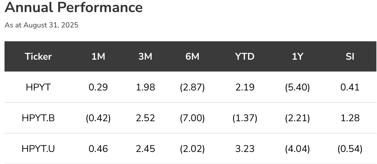
The Harvest Premium Yield Treasury ETF (TSX: HPYT) – a portfolio of ETFs which hold longer dated US Treasury bonds that are secured by the US government, employs up to 100% covered call writing to generate a higher yield and maximize monthly cash flow. It remains in the black in the year-to-date period. HPYT last paid out a monthly cash distribution of $0.13 per unit.
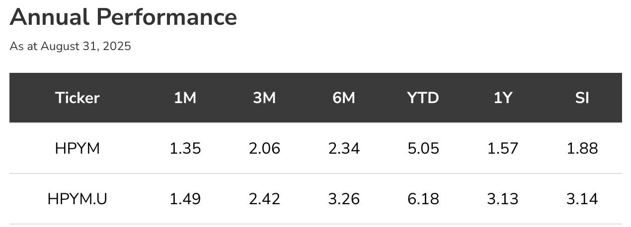
On the medium-term side, the Harvest Premium Yield 7-10 Year Treasury ETF (TSX: HPYM) – a portfolio of US Treasury ETFs that primary hold US bonds with average maturities of 7-10 years. Like HPYT, it can write up to 100% covered call on these holdings to generate monthly income. HPYM has delivered solid returns in the year-to-date period at the midway point in September 2025. The ETF last paid out a monthly cash distribution of $0.08 per unit.
Ambrose O’Callaghan is Senior Copy Writer at Harvest ETFs. Ambrose brings over a decade of experience in the financial services industry to the Content Editor role. He is responsible for providing context to current trends, developments, and analyses to help make sense of the ETF market and emerging themes. With a strong knowledge of the Canadian equity markets and Harvest products, Ambrose regularly provides commentary on a broad array of market topics.
Disclaimer

The content of this article is to inform and educate and therefore should not be taken as investment, tax, or financial advice. Commissions, management fees and expenses all may be associated with investing in Harvest Exchange Traded Funds (managed by Harvest Portfolios Group Inc.). Please read the relevant prospectus before investing. The funds are not guaranteed, their values change frequently, and past performance may not be repeated. The content of this article is to inform and educate and therefore should not be taken as investment, tax, or financial advice.

Certain statements included in this communication constitute forward-looking statements (“FLS”), including, but not limited to, those identified by the expressions “expect”, “intend”, “will” and similar expressions to the extent they relate to the Fund. The FLS are not historical facts but reflect Harvest’s, the Manager of the Fund, current expectations regarding future results or events. These FLS statements are subject to a number of risks and uncertainties that could cause actual results or events to differ materially from current expectations. Although Harvest, the Manager of the Fund, believes that the assumptions inherent in the FLS are reasonable, FLS are not guarantees of future performance and, accordingly, readers are cautioned not to place undue reliance on such statements due to the inherent uncertainty therein. Harvest, the Manager of the Fund, undertakes no obligation to update publicly or otherwise revise any FLS or information whether as a result of new information, future events or other such factors which affect this information, except as required by law.
Dodge costly financial forecasting pitfalls that derail your Financial Independence plans. Canadian retirees need these proven strategies now.
By Dan Coconate
Special to Financial Independence Hub
Planning for Financial Independence requires careful financial forecasting, but many Canadians approaching or already in their golden years make costly errors that jeopardize their financial security.
Understanding common mistakes to avoid in long-term financial forecasts helps protect your hard-earned wealth and maintain the lifestyle you’ve worked decades to achieve.
Ignoring Inflation’s Compounding Impact
Many retirees don’t realize how much inflation can reduce their buying power over time. For example, with just a 2% annual inflation rate, $100,000 today will only be worth about $67,000 in 20 years. In Canada, this is even more concerning as healthcare and housing costs are rising faster than average inflation.
Quick Tips:
Factor 2-4% annual inflation into all projections
Account for healthcare inflation potentially outpacing general rates
Consider variable inflation rates across different expense categories
Overlooking Healthcare Cost Escalation
Provincial health coverage doesn’t eliminate all medical expenses. Dental work, prescription drugs, vision care, and long-term care facilities often involve major costs that many forecasts overlook. These expenses tend to increase with age, potentially leading to budget shortfalls just when you’re least able to return to work, making financial planning essential.
Underestimating Longevity Risk
Life expectancy in Canada continues to rise, with many individuals now living well into their 90s and beyond. This shows the importance of careful financial planning, especially since early retirement may not be sufficient if you live 30 or more years without employment income.
Women, in particular, face unique longevity challenges, often outliving their male partners and needing to manage finances independently for extended periods. Planning is essential to ensure financial stability throughout these longer retirement years.
Using Static Return Assumptions
Market volatility creates sequence-of-returns risk, where poor early performance devastates long-term outcomes despite average returns meeting projections.
A portfolio losing 20% in year one of Financial Independence faces dramatically different outcomes than one gaining 20% initially, even with identical long-term averages.
Managing Market Volatility
Consider dollar-cost averaging withdrawals and maintaining 2-3 years of expenses in conservative investments to weather market downturns without selling equities at depressed prices. Continue Reading…
Flexibility without stock-picking: Sector ETFs offer diversified access to industries like tech, health care, and energy, without the need to select individual companies.
Diversification and precision: Broad ETFs provide market-wide exposure, while sector ETFs let you overweight specific industries based on your market view.
Tactical or strategic: Use sector ETFs for short-term tactical calls or long-term structural tilts (e.g., overweighting defensive sectors for cash flow).
Image courtesy BMO ETFs
By Michelle Allen, BMO ETFs
(Sponsor Blog)
There are many strategies investors can use in their portfolios. One of the most popular strategies is making tactical tilts with sector ETFs.
Sector ETFs – like the new BMO SPDR Select Sector Index range – allow investors to focus on the parts of the market they believe will outperform, such as health care, financials, technology, or industrials.
These ETFs make it simple to increase exposure when certain sectors are expected to perform strongly or dial it back to buffer portfolios when economic conditions change, and are available in both unhedged1 and hedged-to-CAD2 versions.
In this article, we explore how sector behaviours shift across different economic environments, and how tactical tilts using sector ETFs can help investors pursue outperformance.
What is tactical investing?
Tactical investing refers to the process of adjusting portfolio allocations in response to market conditions or economic signals.
While a long-term investor might stick to a static asset allocation, tactical investors“tilt” or increase their exposure toward sectors or asset classes that they believe are poised to outperform over shorter time frames.
Sector ETFs are ideal tools for tactical investing. They allow investors to quickly and easily overweight specific sectors without the need to pick individual stocks. At the same time, they can also be used to create more balanced portfolios as they can be used to diversify portfolios that are concentrated in certain industries.
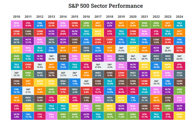
Sector performance can change dramatically each year
Sector performance often mirrors the dynamics seen across different asset classes and individual stocks: the top performers tend to change from year to year as shown in the table below3.
Over the past five years, we’ve seen sectors like information technology, consumer discretionary, and communication services lead the market in 2020 and 2021, only to become some of the worst performers in 2022. That year saw a massive rotation into energy, a sector that had significantly lagged in 2020.
Chart 1 – S&P 500 Sector Performance
Table 1 – S&P 500 Average Sector Returns
Source: Novel Investor (as at March 31, 2025)
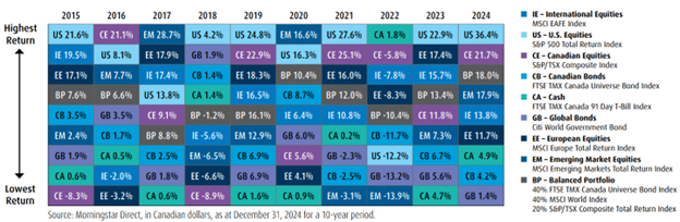
Chart 2 – Asset Class Returns
Index and sector returns do not reflect transactions costs or the deduction of other fees and expenses and it is not possible to invest directly in an Index. Past performance is not indicative of future results.
What drives these rotations? One of the key concepts is the economic cycle, which typically moves through four broad phases:
Recession: A period of economic contraction marked by falling gross domestic product and weak demand.
Recovery: Growth begins to rebound as consumer and business confidence, and spending, return.
Expansion: Economic activity strengthens, employment rises, and output reaches new highs.
Slowdown: Growth decelerates, signaling a potential shift back toward recession.
S&P 500 sector performance during phases
Understanding how sectors behave during different phases of the economic cycle is key to making informed tactical tilts. Here’s a snapshot of average S&P 500 sector performance across the four main stages of the U.S. business cycle (based on historical data from 1960-2019)4: Continue Reading…
John De Goey, a financial advisor and portfolio manager with Designed Securities, and long-time commentator on the financial services industry, was a keynote speaker at The Money Show recently held at the Metro Toronto Convention Centre.
Author of the book ‘Bullshift – How optimism bias threatens your finances’ (Dundurn Press, Toronto, 2023) and host of the popular podcast Make Better Wealth Decisions, De Goey delivered a presentation called Bullshift and Misguided Beliefs.
‘Bullshift,’ the term De Goey has coined, refers to his view about how the financial services industry makes people feel bullish in order to do the industry’s bidding. To make his point, he noted full-page ads appearing in such publications as The Globe and Mail; one of them ran under the headline ‘Be bullish.’
As for misguided beliefs, De Goey says there is ample evidence that Canadian mutual fund registrants believe things which are patently untrue. To illustrate the latter, he referred to Brandolini’s Law.
Alberto Brandolini was an Italian programmer who developed the term in 2013 and his rule goes like this: The amount of energy required to refute BS is an order of magnitude bigger than what was needed to produce it in the first place. Or, put another way, it compares the considerable effort needed to debunk misinformation to the relative ease in creating that misinformation.
American writer and humourist Mark Twain had a take on this at a much earlier time, and De Goey cited that. Said Twain: “It’s easier to fool people than to convince them that they have been fooled.” The point beyond all this, said De Goey, is that people must unlearn what they think they already know. No easy task.
His presentation at The Money Show covered a number of topics including:
The difference between misinformation (an honest mistake) and disinformation (saying something that is deliberately false), and how to unlearn the latter and think for yourself.
How behavioural economics and social psychology affect your investing decisions.
How the industry uses motivated reasoning and tribalism as opposed to critical thinking and evidence.
Why 90% of our financial decisions are based on emotions, not logical thinking.
Why governments and financial advisors like optimism over realism.
De Goey, always a student of history, observed that the market is 30% more expensive now than it was in 1929 just before the stock-market crash that led to the Great Depression. He mentioned the Smoot-Hawley tariffs of 1930 and their catastrophic impact on the U.S. economy, not to mention worldwide economy, and compared this to today’s on-and-off tariffs coming out of the Trump White House. He also noted recent credit downgrades and their effect on the U.S., and, of course, the very real pain of the tariffs which he believes will be much worse in the fourth quarter of 2025. What’s more, De Goey says this will be accompanied by higher inflation.
Bear market looming?
De Goey said the current bull market is “taking its final bow” and the bear market is “waiting in the wings.” In fact, he warned that gains made over the past six years could be entirely wiped out in the next four years if the historical regression to the mean for CAPE occurs. For those who are retired or nearing retirement, this would be devastating news indeed.
One of De Goey’s pet peeves – ‘optimism bias’ – refers to a) people thinking the good times will continue despite blatant warning signs, and b) the very human sentiment that bad things happen but only to other people. Not true, says De Goey. The trouble, he says, is that optimism can sometimes put you in trouble.
Normally, a presentation about money, economics and investing doesn’t get into wisdom imparted by such luminaries as Mark Twain, but De Goey didn’t stop there. He also took a page from Carl Sagan, notably, his 1997 book ‘The Demon-Haunted World. Said Sagan: “If we’ve been bamboozled long enough, we tend to reject any evidence of the bamboozle. We’re no longer interested in finding out the truth. The bamboozle has captured us. It’s simply too painful to acknowledge, even to ourselves, that we’ve been taken. Once you give a charlatan power over you, you almost never get it back.” Continue Reading…