
By Michael J. Wiener
Special to the Financial Independence Hub
How much can we spend from a portfolio each year in retirement? An early answer to this question came from William Bengen and became known as the 4% rule. Recently, Ben Felix reported on research showing that it’s more sensible to use a 2.7% rule.
Here, I examine how a seemingly minor detail, the size of the sampling blocks of stock and bond returns, affects the final conclusion of the safe withdrawal percentage. It turns out to make a significant difference. In my usual style, I will try to make my explanations understandable to non-specialists.
The research
Bengen’s original 4% rule was based on U.S. stock and bond returns for Americans retiring between 1926 and 1976. He determined that if these hypothetical retirees invested 50-75% in stocks and the rest in bonds, they could spend 4% of their portfolios in their first year of retirement and increase this dollar amount with inflation each year, and they wouldn’t run out of money within 30 years.
Researchers Anarkulova, Cederburg, O’Doherty, and Sias observed that U.S. markets were unusually good in the 20th century, and that foreign markets didn’t fare as well. Further, there is no reason to believe that U.S. markets will continue to perform as well in the future. They also observed that people often live longer in retirement than 30 years.
Anarkulova et al. collected worldwide market data as well as mortality data, and found that the safe withdrawal rate (5% chance of running out of money) for 65-year olds who invest within their own countries is only 2.26%! In follow-up communications with Felix, Cederburg reported that this increases to 2.7% for retirees who diversify their investments internationally.
Sampling block size
One of the challenges of creating a pattern of plausible future market returns is that we don’t have very much historical data. A century may be a long time, but 100 data points of annual returns is a very small sample.
Bengen used actual market data to see how 51 hypothetical retirees would have fared. Anarkulova et al. used a method called bootstrapping. They ran many simulations to generate possible market returns by choosing blocks of years randomly and stitching them together to fill a complete retirement.
They chose the block sizes randomly (with a geometric distribution) with an average length of 10 years. If the block sizes were exactly 10 years long, this means that the simulator would go to random places in the history of market returns and grab enough 10-year blocks to last a full retirement. Then the simulator would test whether a retiree experiencing this fictitious return history would have run out of money at a given withdrawal rate.
In reality, the block sizes varied with the average being 10 years. This average block size might seem like an insignificant detail, but it makes an important difference. After going through the results of my own experiments, I’ll give an intuitive explanation of why the block size matters.
My contribution
I decided to examine how big a difference this block size makes to the safe withdrawal percentage. Unfortunately, I don’t have the data set of market returns Anarkulova et al. used. I chose to create a simpler setup designed to isolate the effect of sampling block size. I also chose to use a fixed retirement length of 40 years rather than try to model mortality tables.
A minor technicality is that when I started a block of returns late in my dataset and needed a block extending beyond the end of the dataset, I wrapped around to the beginning of the dataset. This isn’t ideal, but it is the same across all my experiments here, so it shouldn’t affect my goal to isolate the effect of sampling block size.
I obtained U.S. stock and bond returns going back to 1926. Then I subtracted a fixed amount from all the samples. I chose this fixed amount so that for a 40-year retirement, a portfolio 75% in stocks, and using a 10-year average sampling block size, the 95% safe withdrawal rate came to 2.7%. The goal here was to use a data set that matches the Anarkulova et al. dataset in the sense that it gives the same safe withdrawal rate. I used this dataset of reduced U.S. market returns for all my experiments.
I then varied the average block size from 1 to 25 years, and simulated a billion retirements in each case to find the 95% safe withdrawal rate. This first set of results was based on investing 75% in stocks. I repeated this process for portfolios with only 50% in stocks. The results are in the following chart.
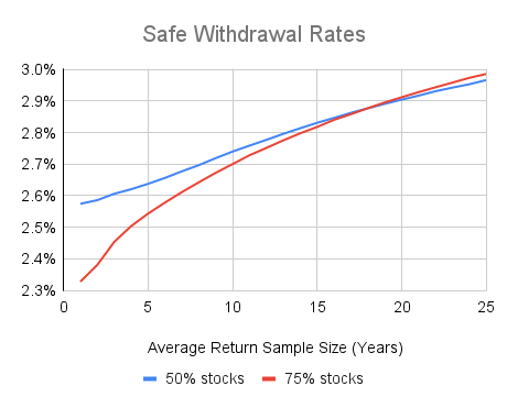
The chart shows that the average sample size makes a significant difference. For comparison, I also found the 100% safe withdrawal rate for the case where a herd of retirees each start their retirement in a different year of the available return data in the dataset. In this case, block samples are unbroken (except for wrapping back to 1926 when necessary) and cover the whole retirement. This 100% safe withdrawal rate was 3.07% for 75% stocks, and 3.09% for 50% stocks.
I was mainly concerned with the gap between two cases: (1) the case similar to the Anarkulova et al. research where the average sampling block size is 10 years and we seek a 95% success probability, and (2) the 100% success rate for a herd of retirees case described above. For 75% stock portfolios, this gap is 0.37%, and it is 0.32% for portfolios with 50% stocks.
In my opinion, it makes sense to add an estimate of this gap back onto the Anarkulova et al. 95% safe withdrawal rate of 2.7% to get a more reasonable estimate of the actual safe withdrawal rate. I will explain my reasons for this after the following explanation of why sampling block sizes make a difference.
Why do sampling block sizes matter?
It is easier to understand why block size in the sampling process makes a difference if we consider a simpler case. Suppose that we are simulating 40-year retirements by selecting two 20-year return histories from our dataset.
For the purposes of this discussion, let’s take all our 20-year return histories and order them from best to worst, and call the bottom 25% of them “poor.”
If we examine the poor 20-year return histories, we’ll find that, on average, stock valuations were above average at the start of the 20-year periods and below average at the end. We’ll also find that investor sentiment about stocks will tend to be optimistic at the start and pessimistic at the end. This won’t be true of all poor 20-year periods, but it will be true on average.
When the simulator chooses two poor periods in a row to build a hypothetical retirement, there will often be a disconnect in the middle. Stock valuations will jump from low to high and investor sentiment from low to high instantaneously, without any corresponding instantaneous change in stock prices. This can’t happen in the real world.
Each time we randomly-select a sample from the dataset, there is a 1 in 4 chance it will be poor. The probability of choosing two poor samples when building a 40-year retirement is then 1 in 16. However, in the real world, the probability of a poor 20-year period being followed by another poor period is lower than 1 in 4. The probability of a 40-year retirement in the real world consisting of two poor 20-year periods is less than 1 in 16.
Of course, by similar reasoning, the simulator will also produce too many hypothetical retirements with two good 20-year periods. So, we might ask whether all this will balance out. The answer is no, because we are looking for the withdrawal rate that will fail only 5% of the time.
Good outcomes from the simulator are largely irrelevant. We are looking for the retirement outcome that is worse than 95% of all other outcomes. When the simulator produces too many doubly-poor outcomes, it drives down this 95% point. The result is an overly pessimistic safe withdrawal rate.
In the more complex case of the simulators discussed here, we are joining return histories of varying lengths, but the problem with disconnects in stock valuations and investor sentiment at the join points is the same. The more join points we have, the more disconnects we create. So, the lower the average return sample length, the lower the safe withdrawal rate result. This is what we saw in the charts above.
In more mathematical terms, the autocorrelations in actual stock prices result in poor periods tending to be followed by above-average periods, and vice-versa. This is called mean reversion. When we select samples from the return dataset and join them together, we partially destroy this mean reversion. The shorter the return samples, the more mean reversion we remove.
Anarkulova et al. selected fairly long samples from their dataset (a decade on average) to try to preserve mean reversion. This helped somewhat, but mean reversion exists on the decade level as well, and choosing 10-year blocks of returns destroys mean reversion between the decades.
What is the remedy?
Anarkulova et al. aren’t misguided in the methods they use. There just isn’t enough available historical return data to run this type of experiment without getting creative. If we had a million years of actual stock returns rather than just a century or so, it would be much easier to determine safe withdrawal rates.
However, we can’t just ignore the problem of properly preserving mean reversion. My best guess is that we need to take the roughly 0.3% gap I observed between Anarkulova et al. approach and the “herd of retirees” approach (described earlier) and add it to the 2.7% withdrawal rate calculated by Anarkulova et al. This gives a base withdrawal rate of 3.0%. Fans of the 4% rule will still find this result disappointingly low, but I believe it is reasonable.
From there a retiree can adjust for other factors. For example, we need to deduct about half the MERs we pay. We also need to spend less if we retire before age 65, and can spend more if we retire after age 65. Another adjustment is that we can withdraw more initially if we are prepared to reduce spending if markets disappoint rather than blindly spend our portfolios down to zero as Bengen’s original 4% rule would have us do. Another adjustment for me is that my total costs (including foreign withholding taxes) on investments outside Canada are lower than the 0.5% assumed by Anarkulova et al. We can make further adjustments if our mortality probabilities are different from the average.
Safe withdrawal rates are a complex area where most of what we read is biased toward telling us we can spend more. Anarkulova et al. used reasonable historical returns and mortality tables to provide an important message that safe withdrawal rates are lower than we may think. However, as I’ve argued here, I think they are too pessimistic.
 Michael J. Wiener runs the web site Michael James on Money, where he looks for the right answers to personal finance and investing questions. He’s retired from work as a “math guy in high tech” and has been running his website since 2007. He’s a former mutual fund investor, former stock picker, now index investor. This blog originally appeared on his site on Dec. 28, 2022 and is republished on the Hub with his permission.